Go has a really nice testing suite built into its compiler tool chains. It's as
simple as running go test in your package, and all files marked *_tests.go
will be executed. We can also run benchmarks during testing, by adding the
-bench flag to the go test command. I never really benchmarked anything
before, so I decided to explore Go's benchmarking utilities, and flex some of my
algorithm skills in the process. Naturally I decided implement the Fibonacci
sequence many, many times over.
The repository lies at https://github.com/TerrenceHo/fib, where you can
use git to clone it. You can also use go get github.com/TerrenceHo/fib
if you have a go runtime, which you'll need to run tests. The file
fib.go holds various fibconacci implementations and some documentation.
The associated tests and benchmarks lie in fib_test.go. To run the benchmarks,
use go test -bench=.. To just run the tests, use go test . My benchmarks are
at the bottom of the article, but we refer to these benchmarks multiple times in
our discussion. I encourage you to try these benchmarks for yourselves.
FibRecursive: Exponential Recursive
func FibRecursive(n int) int {
if n < 2 {
return n
}
return FibRecursive(n-1) + FibRecursive(n-2)
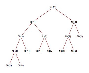
} The most basic Fib sequence algorithm known to man, FibRecursive boasts
a mighty exponential \(O(2^n)\) run time, and is so slow I can't even run
FibRecursive(64) on my laptop without having to wait for an eternity.
The reason being, for an input \(n\), \(n+1\) takes almost twice as long to
computer, since the recursive tree makes two recursive calls each level
and doubles the computation need for the next level.
In our testing suite, we max our runtimecalls at \(n=32\). Memory-wise,
FibRecursive is also inefficient, since each function call
creates adds to the function call stack, and so runs the danger of
actually running out of memory at high inputs.
FibRecursive is clearly unoptimal and so the next few examples of Fibonacci
show slightly more optimized versions.
FibRecursiveCache: Exponential Recursive Cache
func FibRecursiveCache(n int) int {
cache := make([]int, n+1, n+1)
fibRecursiveCache(n, &cache)
return cache[n]
}
func fibRecursiveCache(n int, cache *[]int) {
if n < 2 {
(*cache)[0] = 0
(*cache)[1] = 1
return
}
fibRecursiveCache(n-1, cache)
(*cache)[n] = (*cache)[n-1] + (*cache)[n-2]
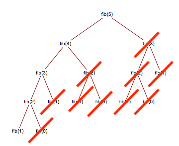
} We notice from the previous expanded FibRecursive tree that many values are
computed many times (i.e. FibRecursive(2) is computed thrice). What if
we compute these values once, and then store it? We can optimize our previous
algorithm by caching previous computed values in an array. In doing so, we
lower our runtime from exponential to linear \(O(n)\), since we cut off most of the
computation tree.
FibRecursiveCache recurses from \(n\) to 1, and then builds the cache
going backwards. The right-most value in our array holds our final answer.
FibRecursiveCache ends up with both a linear runtime and linear memory
usage, due to the array cache.
So where can we improve from here? Let's set aside the runtime optimizations for now, and tackle the memory issue first. If we can get rid of the entire cache, we could save a lot of memeory, since memory is not infinite nor free even on modern computers. The Fibonacci only requires the addition of the two previous terms. So really, we don't need to save all previously calculated Fibonacci values. We can make do with just the previous two, leading us to...
FibIterative: Linear Iterative Implementation
func FibIterative(n int) int {
    var temp int
    first := 0
    second := 1
    for i := 0; i < n-1; i++ {
        temp = second
        second = first + second
        first = temp
    }
    return second
}
FibIterative takes the concept that we do not really need to keep every
previous computed value, only the previous number. Thus we get rid of the
cache entirely and instead add the two previous numbers together in a
loop. This eliminates the need to keep the entire cache in memory, while
keeping the runtime linear, and making the memory required constant.
FibIterative and FibRecursiveCache both have a linear runtime, but
FibIterative performs better on benchmarks, largely due to practical computer
limitations. Performing function calls is slower than iterating through a loop,
since the program must deal with managing the function call stack compared to
simply incrementing a variable. Thus, on my computer anyway, the iterative
implementation is faster.
FibTailRecursive: Tail Recursive Implementation
func FibTailRecursive(n int) int {
    return fibTailRecursive(n, 0, 1)
}

func fibTailRecursive(n, first, second int) int {
    if n == 0 {
        return first
    }
    return fibTailRecursive(n-1, second, first+second)
}
Tail recursion is a trick to place all recursive calls at the end, and do no
more computation after the recursive call returns. This enables the compiler to
reuse the current function call frame and avoid having to create another
(useless) function stack frame. Therefore, tail recursive implementations can be
optimized away by the compiler under the hood into a for-loop implementation.
On benchmarks, FibTailRecursive performs better than FibRecursiveCache, but
still worse than FibIterative. I speculate that memory access and recursive
calls contribute to FibRecursiveCache's worse performace. FibTailRecursive
still has to deal with the very first and last function call, which may explain
the slightly worse performance compared to FibIterative.
Memory wise, FibTailRecursive can be considered to use constant time memory,
because function call frames are not allocated every function call, and
FibTailRecursive does not allocate extra memory, unlike FibRecursiveCache.
Let's see if we can still find a faster implementation for the Fibonacci sequence.
FibPowerMatrix: Linear Matrix Implementation
func FibPowerMatrix(n int) int {
    F := [2][2]int{
        [2]int{1, 1},
        [2]int{1, 0},
    }
    if n == 0 {
        return 0
    }
    fibPower(&F, n-1) return F[0][0]
}

func fibPower(F *[2][2]int, n int) {
    M := [2][2]int{
        [2]int{1, 1},
        [2]int{1, 0},
    }

    for i := 2; i <= n; i++ {
        fibMultiply(F, &M)
    }
}

func fibMultiply(F *[2][2]int, M *[2][2]int) {
    f := *F
    m := *M
    x := f[0][0]*m[0][0] + f[0][1]*m[1][0]
    y := f[0][0]*m[0][1] + f[0][1]*m[1][1]
    z := f[1][0]*m[0][0] + f[1][1]*m[1][0]
    w := f[1][0]*m[0][1] + f[1][1]*m[1][1]

    (*F)[0][0] = x
    (*F)[0][1] = y
    (*F)[1][0] = z
    (*F)[1][1] = w
}
For the unintiated, this algorithm looks a rather complicated. It utilizes \(2 \times 2\) matrix multiplication, and it is not immediately obvious how matrix multiplcation can help solve the Fibonacci sequence. We shall prove the following theorem using induction, where \(F_{n}\) represents the Fibonacci sequence at step \(n\).
\[ M = \left( \begin{array}{ccc} F_{n+1} & F_{n} \\ F_{n} & F_{n-1} \\ \end{array} \right) = \left( \begin{array}{ccc} 1 & 1 \\ 1 & 0 \\ \end{array} \right)^n \]
For \(n=1\),
\[ \left( \begin{array}{ccc} 1 & 1 \\ 1 & 0 \\ \end{array} \right)^1 = \left( \begin{array}{ccc} F_{2} & F_{1} \\ F_{1} & F_{0} \\ \end{array} \right) \]
Which is obvious, these are the first three values in the Fibonacci sequence, \(1, 1, 0\).
Assume that this step holds for \(n=k\).
\[ \left( \begin{array}{ccc} 1 & 1 \\ 1 & 0 \\ \end{array} \right)^k = \left( \begin{array}{ccc} F_{k+1} & F_{k} \\ F_{k} & F_{k-1} \\ \end{array} \right) \]
Now we attempt to prove that the statement still holds for \(n=k+1\), and so the statement would be solved. We multiple both sides by \( \left( \begin{array}{ccc} 1 & 1 \\ 1 & 0 \\ \end{array} \right) \)
\[ \left( \begin{array}{ccc} 1 & 1 \\ 1 & 0 \\ \end{array} \right)^k \left( \begin{array}{ccc} 1 & 1 \\ 1 & 0 \\ \end{array} \right) = \left( \begin{array}{ccc} F_{k+1} & F_{k} \\ F_{k} & F_{k-1} \\ \end{array} \right) \left( \begin{array}{ccc} 1 & 1 \\ 1 & 0 \\ \end{array} \right) \]
\[ \left( \begin{array}{ccc} 1 & 1 \\ 1 & 0 \\ \end{array} \right)^{k+1} = \left( \begin{array}{ccc} F_{k+1} + F_{k} & F_{k+1} \\ F_{k} + F_{k-1} & F_{k} \\ \end{array} \right) \]
This implies that
\[ \left( \begin{array}{ccc} 1 & 1 \\ 1 & 0 \\ \end{array} \right)^{k+1} = \left( \begin{array}{ccc} F_{k+2} & F_{k+1} \\ F_{k+1} & F_{k} \\ \end{array} \right) \]
Thus, by proof by induction, our assumption holds true for any \(n=k+1\). This is basically a simple way to increment the Fibonacci sequence once every matrix multiplcation. We calculate the matrices in a loop, similiar to our tail recursive implementation. Our final answer will be held in the \(F_{k+2}\) after \(n\) iterations.
However, this is still a linear runtime implementation. Worse, since matrix muliplication involves more operations, it is slower than most of our other linear implementations. However, matrix multiplcation opens up a trick to gain a massive speed boost. Memory wise, because we reuse the same matrix, this implementation is constant time.
FibPowerMatrixRecursive: \(Log_n\) Matrix Implementation
func FibPowerMatrixRecursive(n int) int {
    F := [2][2]int{
        [2]int{1, 1},
        [2]int{1, 0},
    }

    if n == 0 {
        return 0
    }
    fibPowerRecursive(&F, n-1) return F[0][0]
}

func fibPowerRecursive(F *[2][2]int, n int) {
    if n == 0 || n == 1 {
    return
    }

    M := [2][2]int{
        [2]int{1, 1},
        [2]int{1, 0},
    }
    fibPowerRecursive(F, n/2)
    fibMultiply(F, F)
    if n%2 != 0 {
        fibMultiply(F, &M)
    }
}
FibPowerMatrixRecursive is pretty similiar to the previous implementation.
However, it uses exponentiation to calculate matrices, rather than simply
multiplying
\( \left( \begin{array}{ccc} 1 & 1 \\ 1 & 0 \\ \end{array} \right) \)
to the previous result
\( \left( \begin{array}{ccc} 1 & 1 \\ 1 & 0 \\ \end{array} \right)^{k} \)
Ignoring matrices for now, consider calculating \(2^8\). We can compute that as \(2 * 2 * 2 * 2 * 2 * 2 * 2 * 2\), and multiple across, which would require 7 multiplication operations. However, you can achieve the same result by using \(4 * 4 * 4 * 4\), since \(2 * 2 = 4\). So we can multiply \(2 * 2\) once to get \(4\), and then use that result to finish the calculation. But we can do that previous step multiple times, and so \(4 * 4 = 16\), \(16 * 16 = 256 = 2^8\). So rather than 7 multiplcation steps, we achieved the same result with 3 steps.
\(2*2 = 4\)
\(4*4 = 16\)
\(16 * 16 = 256\)
This formula is known as the fast exponentiation formula. It brings exponentiation from a linear runtime to a logarithmic runtime, which halves the amount of work every iteration. We can apply the same logic to matrices, squaring the matrices every iteration rather than simply multiplying straight across. In math notation, this would look something like:
\[ \left( \begin{array}{ccc} 1 & 1 \\ 1 & 0 \\ \end{array} \right)^n \left( \begin{array}{ccc} 1 & 1 \\ 1 & 0 \\ \end{array} \right)^n = \left( \begin{array}{ccc} F_{k+1} & F_{k} \\ F_{k} & F_{k-1} \\ \end{array} \right) \left( \begin{array}{ccc} F_{k+1} & F_{k} \\ F_{k} & F_{k-1} \\ \end{array} \right) \]
\[ \left( \begin{array}{ccc} 1 & 1 \\ 1 & 0 \\ \end{array} \right)^{2n} = \left( \begin{array}{ccc} F^2_{k+1} + F^2_{k} & F_{k+1}F_{k} + F_{k}F_{k-1} \\ F_{k+1}F_{k} + F_{k}F_{k-1} & F^2_{k} + F^2_{k-1} \\ \end{array} \right) \]
If \(n\) was odd, then we would multiply once more by \( \left( \begin{array}{ccc} 1 & 1 \\ 1 & 0 \\ \end{array} \right) \)
Because we halve the work necessary each matrix multiplcation, this qualifies as a \(O(log_n)\) implementation. However, that does not mean it's automatically faster than the linear implementations. Due to the overhead in matrix multiplcation, it is actually slower for low values of \(n\), which on my computer was \(n<256\).
In terms of memory usage, because we reuse the same matrices, and do not store all past cached values, the memory usage can be considered linear, with the exception of the recursive calls.
Benchmarks
We test our benchmarks on values \(Fib(n)\), where \(n =
{1,2,4,8,16,32,64,128,256,512,1024}\) (except for FibTestRecursive, we stop at
\(n=32\) because any higher values of \(n\) simply takes too long to run).
Here are the benchmarks on for fib on my computer.
Benchmark Test                        | Iterations | Mean time of operation
---------------------------------------------------------------------------
BenchmarkFibRecursive1-4                1000000000       2.93 ns/op
BenchmarkFibRecursive2-4                200000000        7.77 ns/op
BenchmarkFibRecursive4-4                100000000        22.5 ns/op
BenchmarkFibRecursive8-4                10000000          162 ns/op
BenchmarkFibRecursive16-4               200000           7727 ns/op
BenchmarkFibRecursive32-4               100          17192531 ns/op
BenchmarkFibIterative1-4                500000000        3.50 ns/op
BenchmarkFibIterative2-4                300000000        4.49 ns/op
BenchmarkFibIterative4-4                200000000        6.38 ns/op
BenchmarkFibIterative8-4                100000000        10.3 ns/op
BenchmarkFibIterative16-4               100000000        17.7 ns/op
BenchmarkFibIterative32-4               50000000         39.6 ns/op
BenchmarkFibIterative64-4               30000000         59.9 ns/op
BenchmarkFibIterative128-4              20000000          104 ns/op
BenchmarkFibIterative256-4              10000000          182 ns/op
BenchmarkFibIterative512-4              5000000           351 ns/op
BenchmarkFibIterative1024-4             2000000           673 ns/op
BenchmarkFibRecursiveCache1-4           50000000         31.0 ns/op
BenchmarkFibRecursiveCache2-4           50000000         36.0 ns/op
BenchmarkFibRecursiveCache4-4           30000000         47.4 ns/op
BenchmarkFibRecursiveCache8-4           20000000         68.4 ns/op
BenchmarkFibRecursiveCache16-4          10000000          123 ns/op
BenchmarkFibRecursiveCache32-4          10000000          201 ns/op
BenchmarkFibRecursiveCache64-4          5000000           405 ns/op
BenchmarkFibRecursiveCache128-4         2000000           763 ns/op
BenchmarkFibRecursiveCache256-4         1000000          1514 ns/op
BenchmarkFibRecursiveCache512-4         500000           3091 ns/op
BenchmarkFibRecursiveCache1024-4        200000           6041 ns/op
BenchmarkFibTailRecursive1-4            300000000        5.86 ns/op
BenchmarkFibTailRecursive2-4            200000000        8.63 ns/op
BenchmarkFibTailRecursive4-4            100000000        14.6 ns/op
BenchmarkFibTailRecursive8-4            50000000         27.7 ns/op
BenchmarkFibTailRecursive16-4           20000000         57.7 ns/op
BenchmarkFibTailRecursive32-4           20000000          120 ns/op
BenchmarkFibTailRecursive64-4           10000000          224 ns/op
BenchmarkFibTailRecursive128-4          3000000           438 ns/op
BenchmarkFibTailRecursive256-4          2000000           868 ns/op
BenchmarkFibTailRecursive512-4          1000000          1696 ns/op
BenchmarkFibTailRecursive1024-4         300000           4205 ns/op
BenchmarkFibPowerMatrix1-4              100000000        15.9 ns/op
BenchmarkFibPowerMatrix2-4              200000000        8.05 ns/op
BenchmarkFibPowerMatrix4-4              50000000         32.5 ns/op
BenchmarkFibPowerMatrix8-4              20000000         70.9 ns/op
BenchmarkFibPowerMatrix16-4             10000000          141 ns/op
BenchmarkFibPowerMatrix32-4             5000000           290 ns/op
BenchmarkFibPowerMatrix64-4             2000000           619 ns/op
BenchmarkFibPowerMatrix128-4            1000000          1221 ns/op
BenchmarkFibPowerMatrix256-4            500000           2467 ns/op
BenchmarkFibPowerMatrix512-4            300000           4963 ns/op
BenchmarkFibPowerMatrix1024-4           200000           9599 ns/op
BenchmarkFibPowerMatrixRecursive1-4     200000000        6.24 ns/op
BenchmarkFibPowerMatrixRecursive2-4     200000000        7.44 ns/op
BenchmarkFibPowerMatrixRecursive4-4     100000000        24.8 ns/op
BenchmarkFibPowerMatrixRecursive8-4     30000000         47.9 ns/op
BenchmarkFibPowerMatrixRecursive16-4    20000000         72.6 ns/op
BenchmarkFibPowerMatrixRecursive32-4    20000000         95.5 ns/op
BenchmarkFibPowerMatrixRecursive64-4    20000000          120 ns/op
BenchmarkFibPowerMatrixRecursive128-4   10000000          142 ns/op
BenchmarkFibPowerMatrixRecursive256-4   10000000          166 ns/op
BenchmarkFibPowerMatrixRecursive512-4   10000000          191 ns/op
BenchmarkFibPowerMatrixRecursive1024-4  10000000          213 ns/op
The two noteworthy are BenchmarkFibPowerMatrixRecursive1024-8 and
BenchmarkFibIterative1024-8, which clocked in at 213 ns/op and 673 ns/op,
showing that as \({n\to\infty}\), the \(O(log_n)\) implementation does
indeed scale better. However, at lower values of \(n\), the iterative
implementation should still be used.
Conclusion
Well, we've learned to benchmark programs in Go, and tested out real world implications of complexity analysis. We can achieve real performance gains with the fast exponentiation algorithm, but the overhead in calculating matrices drags the the runtime for lower orders of \(n\). Thus, it can be advisable in real world systems to choose your algorithm depending on the value of \(n\). Good algorithms do really matter after all.